Underfitting and Overfitting

The bias-variance tradeoff explains the relationship between a model’s ability to fit training data and its generalization to unseen data. Striking the right balance between bias and variance is critical for building robust machine learning models.

Empirical Risk and Generalization Gap

Empirical Risk Decomposition

The expected prediction error (empirical risk) for a model \(f̂\) at point \(x\) can be decomposed as:

\[E[(Y - \hat{f}(x))^2] = \underbrace{(E[\hat{f}(x)] - f(x))^2}_{\text{Bias}^2} + \underbrace{E[(\hat{f}(x) - E[\hat{f}(x)])^2]}_{\text{Variance}} + \underbrace{\sigma^2}_{\text{Noise}}\]

where:

• \(f(x)\) is true function

• \(E[f̂(x)]\) is expected prediction

• \(\sigma^2\) is irreducible error

Estimation from Training and Test Errors

Training Error:

\[\text{Train Error} = \frac{1}{n}\sum_{i=1}^n (y_i - \hat{f}(x_i))^2\]

• Underestimates true error due to fitting noise

• Captures part of bias term

• Does not capture variance

Test Error:

\[\text{Test Error} = E_{x,y}[(y - \hat{f}(x))^2]\]

• Includes both bias and variance

• Better estimate of true error

• Independent of training process

Generalization Gap

The difference between test and training error:

\[\text{Gap} = \text{Test Error} - \text{Training Error} = \text{Var}[\hat{f}(x)] + [\text{Bias}^2[\hat{f}(x)] - \text{OptimisticBias}]\]

This shows:

1. Gap directly measures overfitting

2. Training error underestimates true bias

3. Variance contributes fully to gap

Overfitting Characterization

Based on gap magnitude:

\[\begin{split}\text{Overfitting Level} = \begin{cases} \text{None} & \text{if Gap} \approx 0 \\text{Mild} & \text{if Gap} > 0 \text{ and stable} \\text{Severe} & \text{if Gap} \gg 0 \text{ or growing} \end{cases}\end{split}\]

Key insights:

• Underfitting (High Bias):

  • Both training and testing errors are high.

  • The gap between them is small or negligible.

• Overfitting (High Variance):

  • Training error is low, but testing error is significantly higher, creating a large gap.

Practical Applications

1. Model Selection:

   • Choose models minimizing gap while maintaining acceptable training error

   • Use gap trends to guide complexity decisions

2. Training Process:

   • Monitor gap for early stopping

   • Adjust regularization based on gap

   • Balance model capacity against gap size

3. Performance Evaluation:

   • Compare models using both errors and gaps

   • Consider gap stability

   • Account for dataset size effects

Slicing Generalization Gap

Slicing divides the data into subsets based on feature values, residuals, or clusters. This allows for localized analysis of model performance, helping to diagnose underfitting or overfitting in specific regions of the input space.

Define local generalization gap for region \(R\) in feature space:

\[\text{Gap}(R) = E[(Y - \hat{f}(X))^2 | X \in R] - \frac{1}{|R_{\text{train}}|}\sum_{i: x_i \in R} (y_i - \hat{f}(x_i))^2\]

where:

• \(R\) is a region in feature space

• \(|R_{train}|\) is number of training points in \(R\)

Weakness Detection Methods

1. Univariate Partitioning:

For each feature j:

\[R_j^k = \{X: q_k \leq X_j < q_{k+1}\}\]

where:

• \(q_k\) are partitions (or quantiles) of feature \(j\)

• Compute \(Gap(R_j^k)\) for each bin \(k\)

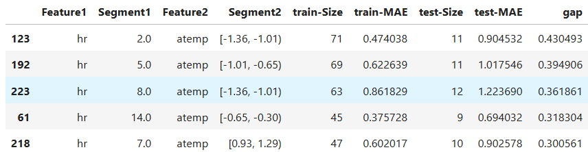
2. Multivariate Region Detection:

Identify high-gap multivariate regions:

\[R_{i,j}^{k,l} = \{X: q_k \leq X_i < q_{k+1}\} \cdot \{X: q_l \leq X_j < q_{l+1}\}\]

where:

• \(q_k,q_l\) are partitions (or quantiles) of feature \(i,j\)

• Compute \(Gap(R_{i,j}^{k,l})\) for each bin \(k,l\)

Identifying Problematic Regions

Flag regions where:

\[\begin{split}\text{Gap}(R) > \text(Threshold) \\text(Threshold) = \mu_{\text{gap}} + \beta \cdot \sigma_{\text{gap}}\end{split}\]

where:

• \(\mu_\text{gap}\) is mean gap across all regions

• \(\sigma_\text{gap}\) is standard deviation of gaps

• \(\beta\) is sensitivity parameter (e.g., 1.5-2)

Overfitting Slicing in MoDeVa

Data Setup

from modeva import DataSet
## Create dataset object holder
ds = DataSet()
## Loading MoDeVa pre-loaded dataset "Bikesharing"
ds.load(name="BikeSharing")
## Preprocess the data
ds.scale_numerical(features=("cnt",), method="log1p") # Log transfomed target
ds.set_feature_type(feature="hr", feature_type="categorical") # set to categorical feature
ds.set_feature_type(feature="mnth", feature_type="categorical")
ds.scale_numerical(features=ds.feature_names_numerical, method="standardize") # standardized numerical features
ds.set_inactive_features(features=("yr", "season", "temp")) # deactivate some features
ds.preprocess()
## Split data into training and testing sets randomly
ds.set_random_split()

Model Setup

# Regression tasks using lightGBM and xgboost
from modeva.models import MoLGBMRegressor, MoXGBRegressor

# for lightGBM
model_lgbm = MoLGBMRegressor(name = "LGBM_model", max_depth=2, n_estimators=100)
# for xgboost
model_xgb = MoXGBRegressor(name = "XGB_model", max_depth=2, n_estimators=100)

Model Training

# train model with input: ds.train_x and target: ds.train_y
model_lgbm.fit(ds.train_x, ds.train_y)
model_xgb.fit(ds.train_x, ds.train_y)

Reporting and Diagnostic Setup

# Create a testsuite that bundles dataset and model
from modeva import TestSuite
ts = TestSuite(ds, model_lgbm) # store bundle of dataset and model in fs
# overfit (gap) slicing for features = season
results = ts.diagnose_slicing_overfit(
   train_dataset="train",
   test_dataset="test",
   features="season",
   method = "quantile",
   metric="MAE",
   threshold=0.0065)
results.table
# To visualize the results
results.plot()

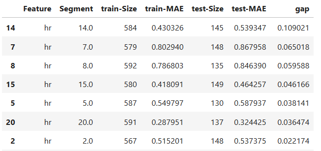
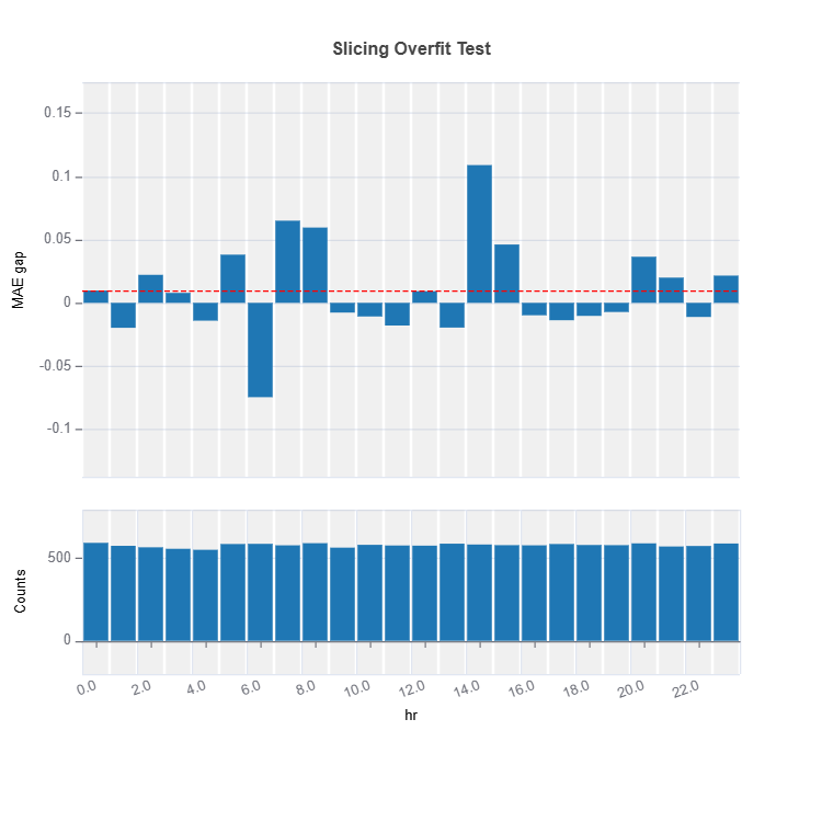
The slicing above is done using “method = quantile” binning with “threshold = 0.0065”. For the full list of arguments of the API see TestSuite.diagnose_slicing_overfit.

Retrieving samples below threshold value

from modeva.testsuite.utils.slicing_utils import get_data_info
data_info = get_data_info(res_value=results.value)["hr"]
data_info

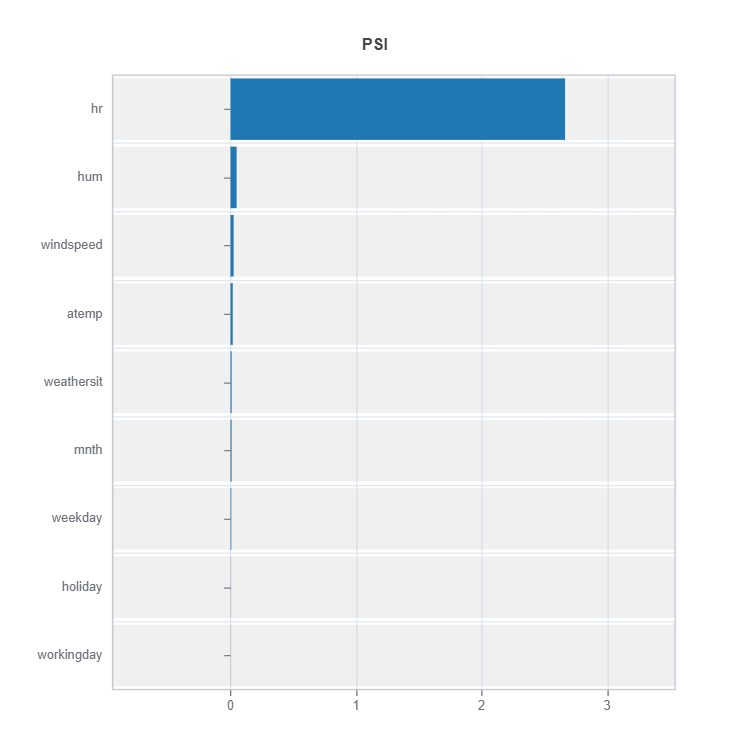
Comparing distribution difference between below and above threshold

data_results = ds.data_drift_test(
   **data_info,
   distance_metric="PSI",
   psi_method="uniform",
   psi_bins=10)
data_results.plot("summary")

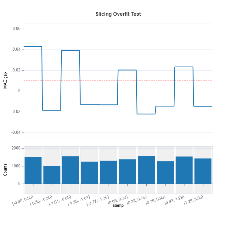
Slicing for a Set of Features with automated binning:

results = ts.diagnose_slicing_overfit(
   train_dataset="train",
   test_dataset="test",
   features=(("hr", ), ("workingday",), ("atemp", )),
   method="auto-xgb1",
   metric="MAE",
   threshold=0.0065)
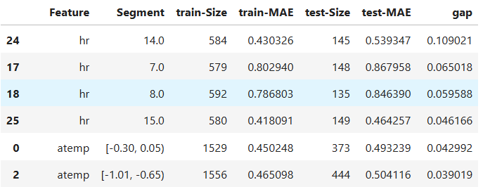
results.table
# To visualize a single feature
results.plot(name="atemp")

2-Feature Interaction Slicing: Two dimensional slicing

results = ts.diagnose_slicing_overfit(
   train_dataset="train",
   test_dataset="test",
   features=("hr", "atemp"),
   method="auto-xgb1",
   metric="MAE",
   threshold=0.0065)
results.table

Overfit Comparison

Slices of several models can be compared as follows:

tsc = TestSuite(ds, models=[model_lgbm, model_xgb])
results = tsc.compare_slicing_overfit(
   train_dataset="train",
   test_dataset="test",
   features="hr",
   method="quantile",
   bins=10,
   metric="MAE")

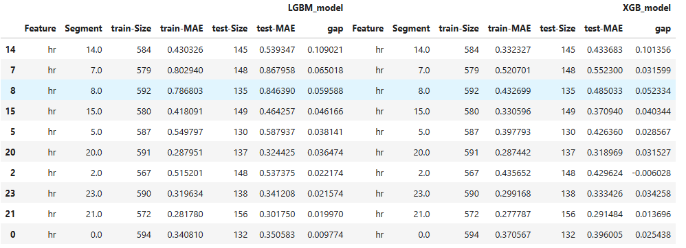
Check the API reference for detail arguments of TestSuite.compare_slicing_overfit.

Characterization of Weak Regions

1. Data Sparsity:

\[\text{Density Ratio}(R) = \frac{|R_{\text{test}}|/|{\text{test}}|}{|R_{\text{train}}|/|{\text{train}}|}\]

2. Complexity Measure:

\[\text{Local Complexity}(R) = \text{Var}[\hat{f}(X) | X \in R]\]

3. Uncertainty Assessment:

\[\text{Uncertainty}(R) = \text{Std}[(Y - \hat{f}(X))^2 | X \in R]\]

Overfitting and Model Robustness

MoDeVa provides robustness test capability. Robustness measures a model’s ability to maintain performance when subjected to input perturbations or noise. The detail description of the robustness test can be found in the robustness testing section.

The relationship between overfitting and robustness can be understood through the lens of local Lipschitz continuity:

\[|f(x + \delta) - f(x)| \leq L||\delta|| \text{ for small } \delta\]

Theoretical Framework

1. Gradient Sensitivity:

For an overfit model:

\[||\nabla f(x)|| \text{ tends to be larger} \implies \text{Higher sensitivity to perturbations}\]

2. Local Curvature:

\[\text{Overfitting} \rightarrow \text{Higher Local Curvature} \rightarrow \text{Larger } ||\nabla^2 f(x)||\]

3. Generalization Gap Connection:

\[E[|f(x + \delta) - f(x)|] \approx ||\nabla f(x)|| \cdot E[||\delta||] \text{ correlates with gap size}\]

Manifestations

1. Decision Boundary Complexity:

   • Overfit models → Complex, wiggly boundaries

   • More sensitive to small perturbations

   • Higher local Lipschitz constants

2. Feature Sensitivity:

   • Overfit models rely heavily on noise

   • Small changes have larger effects

   • Less stable predictions

3. Neighborhood Consistency:

   • Robust models → Similar predictions for similar inputs

   • Overfit models → More erratic local behavior

   • Affects adversarial robustness

Remediation Strategies for Model Weaknesses Identified by Gap Analysis

Data-Centric Solutions

1. Targeted Data Collection:

For regions \(R\) with large gaps:

\[P(X_{\text{new}} \in R) \propto \text{Gap}(R)\]

Approaches:

• Active learning in high-gap regions

• Stratified sampling based on gap size

• Domain expert data collection

2. Data Cleaning:

• Remove noisy samples in high-gap regions

• Validate labels in problematic areas

• Handle outliers affecting local gaps

Feature Engineering Solutions

1. Interaction Features:

Create new features for high-gap regions:

\[f_{\text{new}} = g(X_i, X_j) \text{ where } (i,j) \in \text{high-gap pairs}\]

2. Domain-Specific Transformations:

\[X_{\text{transformed}} = h(X) \text{ based on } \text{Gap}(R)\]

Examples:

• Log transforms for skewed features

• Binning for nonlinear relationships

• Feature combinations based on domain knowledge

• Apply constrainst such as monotonicity

3. Feature Selection:

Weight features by gap reduction:

\[w_i = -\frac{\partial \text{Gap}(R)}{\partial X_i}\]

Model-Centric Approaches

1. Select alternative modeling frameworks

2. Local Model Enhancement:

\[\begin{split}f_{\text{enhanced}}(X) = \begin{cases} f_{\text{local}}(X) & \text{if } X \in R_{\text{weak}} \f_{\text{global}}(X) & \text{otherwise} \end{cases}\end{split}\]

3. Ensemble Strategies (Mixture of Experts):

\[f_{\text{ensemble}}(X_i) = \sum_{k} w_{k,i}(X_i)f_k(X_i)\]

where:

• \(w_{k,i}(X)\) higher in high-gap regions

• \(f_k\) specialized for different regions

Apply Mixture of Experts (MoE) model with proper regularization. The detail description of the MOE can be found in the moe section.

4. Loss Function Adjustments

1. L1/L2 Regularization:

L1 Regularization (Lasso):

\[L_{\text{total}} = L_{\text{pred}} + \lambda_1 \sum_{i} |w_i|\]

Properties:

• Promotes sparsity

• Helps feature selection

• May be too aggressive in high-sensitivity regions

L2 Regularization (Ridge):

\[L_{\text{total}} = L_{\text{pred}} + \lambda_2 \sum_{i} w_i^2\]

Properties:

• Smooths decision boundaries

• More stable than L1

• Might not address local sensitivity issues

2. Gap-Weighted Loss:

\[L_{\text{new}}(X,y) = L_{\text{original}}(X,y) \cdot (1 + \alpha \cdot \text{LocalGap}(X))\]

3. Region-Specific Penalties:

\[L_{\text{total}} = L_{\text{pred}} + \lambda \sum_{R \in \text{weak}} \text{Penalty}(R)\]

Implementation Framework

1. Prioritization:

   • Rank regions by gap size

   • Assess feasibility of each solution

   • Consider implementation cost

2. Validation:

   • Monitor gap reduction

   • Check for negative side effects

   • Validate on holdout set

3. Iteration:

   • Start with simplest solutions

   • Gradually add complexity

   • Monitor impact on overall model

The bias-variance tradeoff highlights the balance between underfitting and overfitting. By analyzing the gap between training and testing errors and applying slicing techniques to evaluate performance across subsets, practitioners can diagnose specific issues and improve model reliability. Striking the right balance ensures optimal generalization and robust predictions for unseen data.

Examples

Example 1: Bike Sharing

The example below demonstrates how to use MoDeVa with its high-code APis for the Bike Sharing dataset from the UCI repository, which consists of 20,640 samples and 9 features, fetched by sklearn.datasets. The response variable MedHouseVal (Median Home Value) is continuous and is a regression problem.

• Overfitting Analysis (Regression)

Examples 2: Taiwan Credit

The second example below demonstrates how to use MoDeVa’s high-code APIs for the TaiwanCredit dataset from the UCI repository. This dataset comprises the credit card details of 30,000 clients in Taiwan from April 2005 to September 2005, and more information can be found on the TaiwanCreditData website. The FlagDefault variable serves as the response for this classification problem.

• Overfitting Analysis (Classification)