Model Test

The Model Test panel enables the evaluation of model performance across four key dimensions: Performance, Reliability, Robustness, and Resilience.

Initialize the Panel

To create and initialize the Model Test panel, use:

# Load the Experiment and test a model
from modeva import Experiment
exp = Experiment(name='Demo-SimuCredit')
exp.model_test()

Workflow

Step 1: Select Dataset & Model

1. Select a Dataset: The dataset from the dropdown for processing is automatically selected based on the processed dataset of the experiment (e.g., Demo-SimuCredit_md).

2. Set the Data Selection: Choose a data split (e.g., test).

3. Set Select Model: Pick a registered model from the dropdown (e.g., XGBoost).

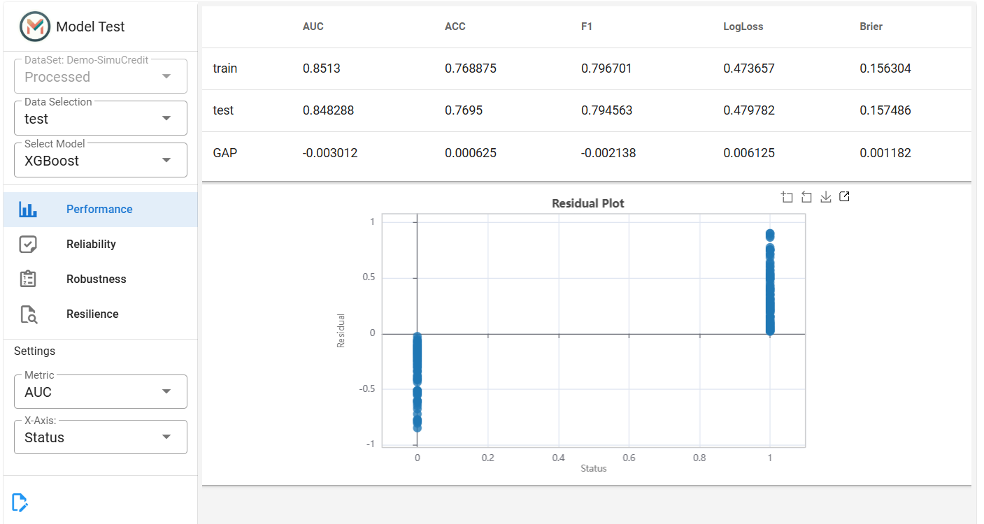
Step 2: Performance Evaluation

1. Select Evaluation Metric:

   • Choose a task-specific metric (e.g., MSE for regression, AUC for classification).

2. Residual Analysis:

   • Select a feature for the X-axis to visualize prediction residuals.

3. View Outputs:

   • Summary Table: Displays key accuracy metrics.

   • Residual Plot: Visualizes residuals against the selected feature.

Step 3: Reliability Testing

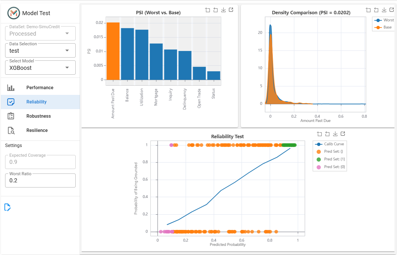
1. Configure Settings:

   • Expected Coverage: Define confidence interval width (e.g., 0.9 for 90% coverage).

   • Worst Ratio: Set the acceptable error threshold (e.g., 0.1).

2. View Outputs:

   • Calibration Plot: Compares predicted vs. actual confidence intervals.

   • Distribution Shift (PSI): Assesses data stability between training and test sets.

Step 4: Robustness Testing

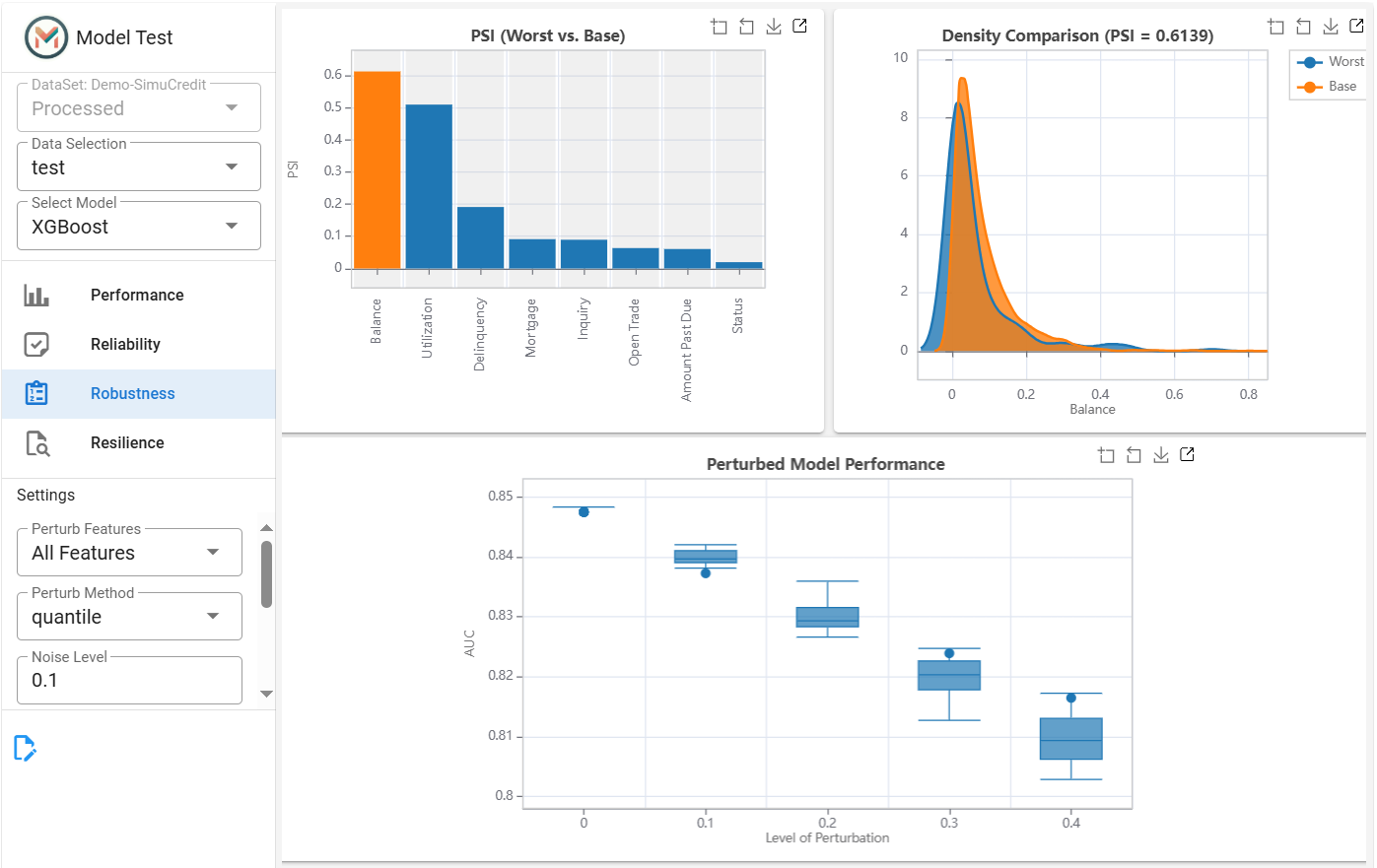
1. Configure Perturbations:

   • Features: Select features to perturb (e.g., Mortgage).

   • Method: Choose quantile (distribution-based) or normal (Gaussian noise).

   • Noise Level: Define perturbation strength (e.g., 0.1).

2. View Outputs:

   • Robustness Plot: Displays performance degradation under noise.

   • Locate Features: Identifies features with the most significant distribution shift on prediction changes after perturbation.

   • Distribution Shift: Click the bar of interest from the PSI bar plot to view the feature distribution shift between base and worst samples.

Step 5: Resilience Testing

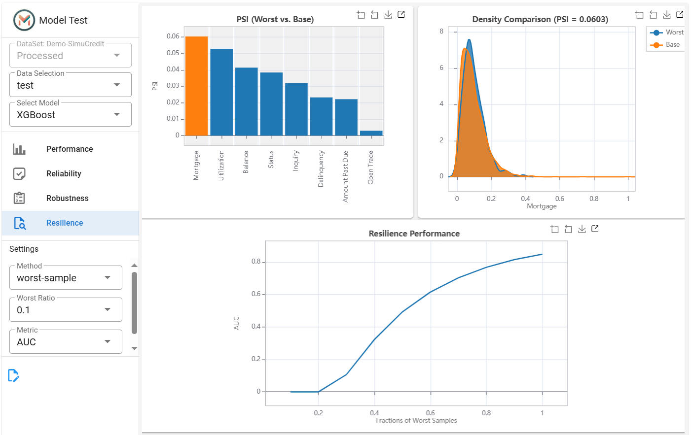
1. Configure Settings:

   • Method: Select worst-sample (identifies hard samples) or outer-sample (boundary samples).

   • Worst Ratio: Define the proportion of worst-case samples (e.g., 0.1).

2. View Outputs:

   • Resilience Plot: Displays performance degradation on challenging samples.

   • PSI Plot: Identify features with the most significant distribution shift on performance.

   • Distribution Shift: Click the bar of interest from the PSI bar plot to view the feature distribution shift between base and worst samples.

Step 6: Saving Results

• Click the |register_icon| button to save test results.

This panel provides actionable insights into model behavior under real-world conditions. For advanced analysis, use the linked distribution visualizations to drill into specific features. For more information, refer to the Diagnostic Suite.